The FarmAC model simulates the flow of carbon (C) and nitrogen (N) on arable and livestock farms, enabling the quantification of greenhouse gas emissions and N losses to the environment. The model uses a mixture of Tier 2 (emission factor) and Tier 3 methodologies, and relies on inputs that should be available to educated, competent farmers or farm advisors. The model can be used to investigate a range of management options designed to compensate for negative effects of climate change or take advantage of positive effects. This is achieved by the user designing a baseline scenario and then one or more additional management scenarios.

This document is designed for model users. The model requires parameterisation by local experts for each agro-climatic zone and a separate user guide is available for these local experts.

FarmAC is designed to be a flexible and adaptable model. This means that it can be used to describe a wide range of global farm systems. However, when using the model, it is important to remember that this flexibility and adaptability is obtained at a price. That price is that the users have the responsibility to assure themselves that their inputs are realistic. The model will report an error if it detects that some impossible situations have arisen. For example, if user inputs would mean the commitment of more than 100% of the C or N available. Furthermore, the model checks whether the production of grazed roughage matches the consumption indicated by the user. However, there are no other reality checks, so users need to ensure in particular that:

· Livestock are capable of consuming the feed ration input.

· The qualities of the crop products are realistic, relative to the fertilisation. This is particularly important for roughage crops such as grass, since the protein content of roughage crop products varies significantly in response to fertilisation.

· When investigating different scenarios for farm management, the user must ensure that the distribution of the farm area between soil types is the same as in the baseline scenario.

3 Model function

The model describes the flow of carbon (C) and nitrogen (N) on a farm. The main flows and losses for C and N are shown in Figs 1 and 2.

Fig 1 C flows

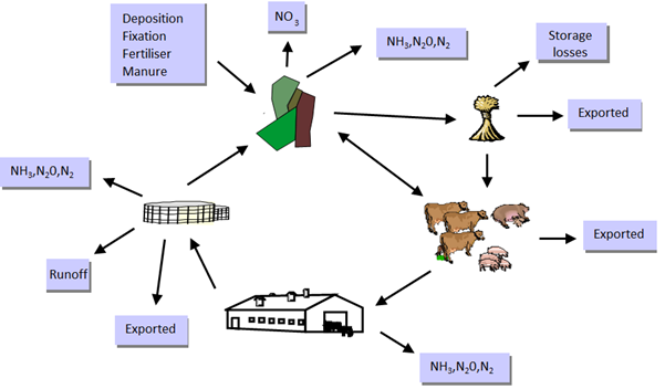
Fig 2 N flows

Much of FarmAC functions in a similar way as other nutrient budgeting tools (e.g. carbon calculators, farm N surplus tools). The fate of C and N input to the farm is followed until it leaves the farm again, either within agricultural products (including manure) or is lost to the environment. However, FarmAC differs with respect to the treatment of the soil. A dynamic soil model is used in which the transformations of C, N and H₂O are followed over time, with timescales ranging from days to centuries. This enables the model to take account of two important features:

· The effect of previous land use and management on changes in the amount of C and N stored in the soil, and the availability of N for plant growth.

· The carryover effect of mitigation and/or adaptation measures e.g. the effect of introducing cover cropping or changes in the management of crop residues on the production and losses from subsequent crops.

However, the advantages of using a complex soil model are obtained at a price; the model contains more parameters that must be evaluated, more input data are required and the results are less easily interpreted than would be the case if a more simple or no soil model were included. Furthermore, the user needs to consider which of the following two situations best describes their conditions:

1. Farming systems where there has been no dramatic changes in land use in the past hundred years (e.g. from forest to agricultural land) and the cropping practice and management has been relatively stable over the recent past 50 years (e.g. has been grassland or arable during this period). Here we can assume that the soil C pools of interest are largely in equilibrium with the inputs of crop residues and animal manure.

2. Farming systems where there has either been a change in land use in the past hundred years (e.g. from forest to agricultural land) or a substantial change in the cropping practice and management over the past 1-50 years (e.g. from grassland to arable or the reverse). Here we must assume that the soil C pools of interest are not in equilibrium with the inputs of crop residues and animal manure.

‘Substantial’ changes in management mean large changes in the balance between the grass and arable crops grown or large changes in the level of fertilisation/manuring. If in doubt, choose Case 1. Guidance on how to use the model for Case 1 is given in the following section whereas guidance for Case 2 is shown in? For Case 1, a baseline scenario must be defined i.e. a farm must be defined that describes the current structure and management. The model must then be run for a long adaptation time period (typically several centuries) to allow the soil model to equilibrate with the current structure and management. The model is then run for a much shorter projection period (typically <20 years) to allow the current C and N flows to be calculated. Thereafter, the user has the option to create new scenarios in which the structure and/or management of the farm is changed. These scenarios are then simulated for the projection period, with the soil model initialised using the results from the baseline adaptation simulation. The results of simulating these scenarios can then be compared with those obtained when simulating the baseline scenario for the projection period.

Finally, another feature of FarmAC is that for non-grazed feed items, any difference between consumption by livestock and on-farm production is balanced by farm imports or exports. However, grazed roughage cannot be imported or exported so when considering ruminant livestock farms, it is the responsibility of the user to ensure that the production and consumption of such roughage (including grazed crop residues) are in balance.

4 Using the user interface – entering data

4.1 Overview

The user interface is Internet based i.e. data input and output occurs via an Internet browser. On start-up, the user is asked to select a farm to be modelled. They can choose to create an empty farm to which they will then have to add farm components or choose to create a copy of a farm from a list of existing model farms (either standard farms or farms created earlier by the user) and edit this to describe a new farm. There is also an option to delete an existing farm.

The user is then presented with a web page containing a number of tabs:

· The Farm collects general information concerning the farm.

· The Cropping sequence tab collects information concerning the crops planted and the details of the crop products generated.

· The Yield tab collects information concerning the DM yield and the purpose to which this yield is put.

· The Ruminants and Non-ruminants tabs collect information concerning the number and type of livestock present, their feed rations, their housing and the type of manure storage.

· The Manure tab is used to enter information concerning the amount and type of manure and fertiliser applied to each crop, together with information on the application method.

The first task is to define a baseline scenario. Information should normally be input in the order Farm - Cropping sequence -Yield - Ruminants - Manure, since grazed feed items are only available for inclusion in the diet of ruminants if the user interface detects that they are grown on the farm and organic manures are only available for application to crops if the user interface detects that they are either imported or produced on the farm. Once a baseline scenario has been defined and successfully simulated, the user is then free to define one or more additional scenarios in which the effect of changes to the farm structure or management can be investigated.

4.2 Accessing the interface

To access the interface and use the model, it is necessary to have a user account. This currently requires sending an emailed request to nick.hutchings@agro.au.dk. New users will receive an email containing a user name and password, plus a URL address that allows the interface to be accessed using an Internet browser (e.g. Firefox). This webpage should look as follows:

Fig 3 Login webpage

Enter the user name and password and the following webpage appears.

Fig 4 Farm choice webpage

The user can then choose from the following options:

· To create a new, empty farm.

· To make a copy of one of the user’s existing farms.

· To delete one of the user’s existing farms.

· To create a copy of a standard farm.

The standard farms are currently a collection of simple test farms (created during the development of the model) and model farms created during the AnimalChange project.

4.2.1 Switching between farms or logging out

When the choice has been made, the user interface webpage will appear. This contains a number of tabs (see below). The links Select farm and Log out are available at all times on the first line of the user interface webpage. The Select farm link returns the user to the Farm choice webpage (Fig 4) whereas the Log out link will log the user out and return them to the Login webpage (Fig 3).

4.3 Farm tab

You can choose between creating a new farm from an empty farm or by modifying a copy of an existing farm. It is often easier to modify a copy of an existing farm. New users will not have existing farms that can be copied but can choose to copy a standard farm.

If you begin with an empty farm, you will see the following:

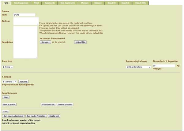
Fig 5 Farm webpage

This tab enables the user to describe the farm in general terms, set some general parameters and input some farm-scale inputs (Table 1).

Table 1 Farm data inputs for Farm tab

User input	Description	Note
Farm type	The dominant type of farming practiced in the past 10 – 20 years.
Agro ecological zone	Choice of Agro ecological zone	Choose a standard zone from the drop-down box
Atmospheric N deposition	Annual deposition of N from the atmosphere (NOT biological N fixation)	Livestock density of region: High = 40 Medium = 25 Low = 5

Remember to press Save. Provided you do this, the data you have entered will be saved for later use. This is particularly important if you are interrupted while you are entering data, since the user interface will log you out if you have been inactive for more than 5 minutes. If this happens, you will need to log on again and select your farm from the dropdown box.

If the user wishes to use one or more farm-specific parameter files, these can be uploaded or deleted from this tab.

The tab contains a number of buttons:

· Rename allows a scenario to be renamed.

· New, Copy or Delete Scenario; New will create a farm with no structure, Copy will create a copy of the current scenario and Delete will delete the current scenario. All farms need one and only one baseline scenario. This scenario must have the key text ‘baseline’ or ‘Baseline’ in its name. Use the Rename button to do this.

· Run the model in Adaptation mode; this runs the model for a long period*, to allow the soil model to adapt to management. This button should only be used for baseline scenarios.

· Run model Projection; this runs the model for a short period (usually some decades). The model results displayed on the interface are the average of the results for these years.

· Create xml; this is only used to enable users that run the model on their own PC to generate an input file.

* often 50 years or more.

Furthermore, the tab allows users to create, copy or delete scenarios. Users will normally be advised to create and test the baseline scenario first. When investigating mitigation or adaptation measures, one or more additional scenarios can then be created by copying the baseline scenario and then making the (often minor) changes in structure or management.

If manure is imported into the farm, the New Bought manure allows the user to indicate that manure should be imported. This requires then additional input (see Table 2).

Table 2 Data inputs for Bought manure

User input	Description	Note
Bought manure type	Type of manure imported to the farm. This only appears if the user clicks on the New bought manure button

4.4 Cropping sequence tab

The Cropping sequence tab allows the user to define a variable number of crop sequences. If the farm is landless, the user must check the tickbox to confirm this.

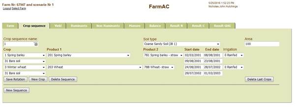
Fig 5 Example cropping sequence for arable cropping

Choose the soil type and the area. It is optional whether you change the name of the crop sequence to something more meaningful to you. One crop will be added automatically. Change this to a crop of your choice and edit its start and end date. If relevant, choose the type of product or products that the crop creates. Choose whether the crop is rainfed or irrigated.

A crop sequence must last at least one year (365 days) and the day and month on which the last crop ends must be one day before the day and month of the start of the first crop. Note that the date of the last crop in the sequence must be one day before the first day of the first crop (e.g. if the first crop starts on 2.4.20xx then the last crop must end on 1.4.20yy). If there is a period with bare soil between crops, add this period as if it too were a crop. There can be no gaps in the cropping sequence. For example, if there is only one crop (e.g. permanent grass), this could have a start date of 01.04.2001 and an end date of 31.3.2002. Note that the starting year chosen is irrelevant (the model will set this to be Year 1 and 2002 to be Year 2). In the example shown below, the sequence starts on 2 March and finishes on 1 March, two years later. Thereafter, crops are added in order with which they are grown. Cover crops are input in the same way as other crops. The data that can be entered by user is shown in Table 3.

Table 3 Data inputs for each Cropping sequence

User input	Description
Total area of rotation	Area of rotation in ha
Soil type	Dominant soil type in rotation
Irrigation	Indicate if irrigation of each crop is performed
Crop grown in year n	Relevant crop types
Primary product from crop grown in year n	Types of primary crop product (e.g. wheat grain, high quality silage)
Secondary product from crop grown in year n	Type of secondary crop product (e.g. wheat straw, fodder beet tops)
Starting date for crop n*	Day, Month, Year
End date for crop n	Day, Month, Year

* normally the sowing date. However, for undersown crops (e.g. grass undersown in a cereal crop), the starting date is equated to the end date of the main crop.

The minimum length of the crop sequence is one year whereas the maximum length is variable, provided it is an exact number of years and does not exceed the simulation period specified in the model parameterisation. If the length of the crop sequence is less than the simulation period, the sequence will be repeated (Fig 6).

Fig 6 Schematic representation of a four-year cropping sequence

This means that the sequence of crops must be continuous i.e. if crop x finishes on day 1, crop x+1 must start on day 2. It also means that the last crop in the sequence must finish one day before the starting date of the first crop. Note that the exact year when a crop sequence commences is irrelevant but the cropping years thereafter need to be in sequence i.e. the model will treat cropping sequences with periods 1970 to 1975 or 2000 to 2005 identically (they would both be converted to year 1 to 5). Different cropping sequences can have different durations.

Depending on the crop chosen, the interface may allow the user to select crop Product 1 or 2 from a list of products of differing qualities. Each crop product has a set of quality characteristics (defined in a parameter file) that includes the N concentration. Since the dry matter (DM) production is determined by the N available to the crop, the higher the N concentration in a crop product, the lower will be the DM production.

4.4.1 Temporary and permanent crops

The assumption in the model is that temporary crops are sown on their starting date and are harvested on their end date. This assumption affects the timecourse of some aspects of the soil water model (rooting depth and leaf area) and the input of crop residues to the soil C and N model. A different timecourse is appropriate for permanent crops such as permanent grass or forest trees, since these crops do not have an establishment phase. To enable this distinction to be made, the model treats crops with a name containing the word ‘permanent’ as permanent crops and all other crops are treated as temporary.

It is often advisable to describe a permanent crop using more than one crop, since this allows a more accurate representation of management and growth conditions. An example is shown in Fig 7, where a permanent grass crop only grazed during the growing season. This way to describe the crop sequence would result in the excreta from grazing livestock being deposited on the crop only during the growing season and would result in a proportion of out-of-season grass growth to be returned to the soil as crop residue.

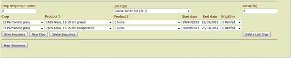
Fig 7 Example of splitting a permanent forage crop between two crops

4.4.2 Arable crops

For arable crops, there may be one or two crop products. For example, a cereal crop grown to maturity (Fig 5) will produce both a main product (grain) and a secondary product (straw), whereas a cereal crop grown for silage will only produce one main product (whole-crop silage). If a cover crop is grown in the period between the harvesting of one arable crop and the sowing of the next, the cover crop is input as a separate crop, starting on the day following the harvesting of the cereals (Fig 8). Note that for the cover crop, the crop product is indicated as being incorporated. This means that the crop product will not be harvested but its biomass will be added to the soil.

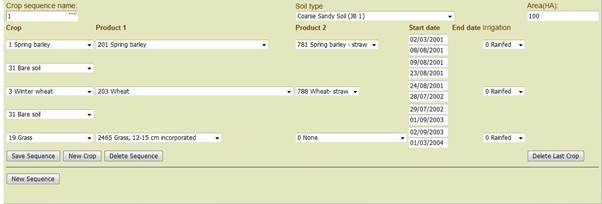
Fig 8 Example of a cereal cropping sequence with a grass cover crop

4.4.3 Grass and other forage crops

With the exception of forage crops grown for seed (which are treated as for a cereal crop), forage crops are treated as a special case. The quality and production of some forage crops (e.g. grass) depends a great deal on how it is utilised (particularly grazing versus cutting). Several situations can be envisaged:

· If the whole of a forage crop is utilised by a mixture of grazing and harvesting throughout the growing season but is subject to one manure and fertiliser management regime, two separate crop products (one harvested and one grazed) should be defined (Fig 9).

· If the whole of a forage crop is utilised first by one method (grazing or harvesting) and later by one or more other method, the crop should be defined as two (or more) separate crops (e.g. Fig 10).

· If part of a forage crop is harvested by the same method all season and the other part is harvested by a mixture of methods, often with differences in fertiliser and manure management, the situation should be described by defining two cropping sequences (e.g. Fig 11).

Fig 9 Defining a crop sequence where the whole of a forage crop is utilised by a mixture of grazing and harvesting for silage throughout the growing season.

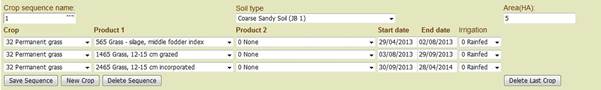
Fig 10 Defining a crop sequence where a forage crop is harvested first for silage and then by grazing.

Fig 11 Defining a crop sequence where a forage crop is managed as two distinct areas.

4.5 Yield tab

The sequence entered in the Cropping sequence tab is reproduced here. If the farm is landless, this tab will not be accessible.

The potential production (i.e. unlimited by water or N supply) of each crop product must be entered (Fig 12). Remember:

· This potential production is per period and not per year.

· Unless the crop is well supplied with fertiliser and water, this is not the yield that is commonly achieved. The model itself will calculate the actual yield from the potential yield, taking account of the availability of water and N. If this occurs and the crop has two crop products, the DM yield of each crop product is reduced by the same proportion i.e. the relative distribution of DM between the two products remains the same.

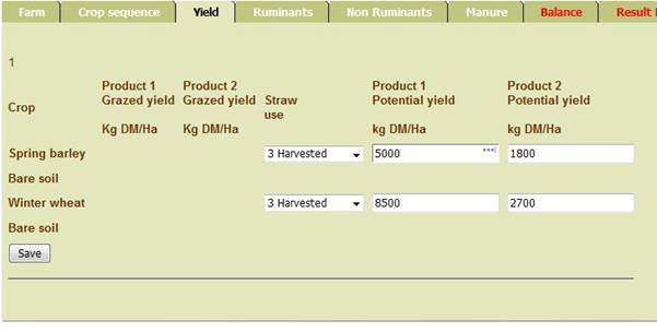
Fig 12 Yield tab for an arable crop sequence

The Straw use dropdown box (if visible) is used to indicate the fate of any straw produced (Table 4). For grazed forage crops, there are additional text boxes; the value entered in the Grazed yield text boxes represent the DM yield that will be consumed by grazing.

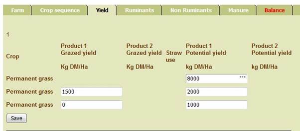
Fig 13 Yield tab for a cropping sequence with grazed grass.

Here you can see that the annual potential DM yield for the permanent grass has been set at 11000 kg ha^-1. In the first crop sequence, this potential is divided between grass grown for silage (8000), between grass grown for grazing (2000) and the grass that will contribute to the DM deposited onto the soil as crop residues over winter (1000). The actual production of silage will depend on the availability of water and N during the growing season. The actual grazed grass production is 1500 kg ha^-1. This production must be achieved or the model will report an error. If the production exceeds this value, the surplus will contribute to crop residues. The actual production of grass that will contribute to the DM deposited onto the soil as crop residues over winter will depend on the availability of water and N over the winter.

Table 4 Data inputs for each crop

User input	Description
Potential DM production of primary product (Product 1)	Dry matter yield (t ha^-1)
Potential DM production of secondary product (Product 2)	Dry matter yield (t ha^-1)
Fate of the secondary product	see Table 5
Product 1 yield	Actual dry matter yield to be achieved (t ha^-1)
Product 2 yield	Actual dry matter yield to be achieved (t ha^-1)

Table 5 Choices for the fate of secondary crop products

Choices presented	Fate of secondary product	Notes
Harvested	Straw is harvested and removed from field. Stubble is incorporated in the soil surface at harvesting time.	Available for all crops that produce straw
Incorporated	As for Harvesting (incorporation to depth not currently implemented)	Available for all crops that produce straw
Burnt	All straw is burnt; no stubble remains to be incorporated in soil
Burnt stubble	Straw is harvested and removed from field. Stubble is burnt.
Residue grazed, stubble burnt	Straw remains as a residue and is grazed during the subsequent crop. Any residue remaining ungrazed is burnt	Only available if the subsequent crop is bare soil
Residue grazed, stubble left	Straw remains as a residue and is grazed during the subsequent crop. Any residue remaining ungrazed is incorporated in the soil surface	Only available if the subsequent crop is bare soil
Residue grazed, stubble incorporated	As for Residue grazed, stubble left	Only available if the subsequent crop is bare soil

4.6 Ruminants tab

This tab is used to enter details of the ruminants present on the farm. Ruminant types are added by clicking on the New button. For all types of ruminant, the information to be entered includes the number present, details of the feed ration (the type and dry matter amount of each feed item (Fig 14, Table 6). When the user enters a feed item to the feed ration, a new drop-down box will appear. The crop products that are produced on the farm are marked with a green background, for easier identification and selection. Remember to click the Save button occasionally, so if anything goes wrong, you have saved your data.

Note that the number of animals is expressed as the annual average population (as is also used by IPCC). This is equivalent to the average number of animals present as determined by a representative census. Often it is advisable to divide a herd or flock into several groups, each reflecting animals with different feed rations. For example, it is often advisable for cattle to define one group that has a summer/dry season ration and another than has a winter/wet season ration. The equation for calculating the number of animal to enter into the user interface depends on how they are counted. If they are counted by census (= annual average population), the calculation is:

number in group y = (z/12) * annual average population

where z is the number of months the animals are on the particular feed ration.

If instead the animals are counted in terms of the number produced, the calculation is:

number in group y = (s/12) * (z/12) * annual average population of the livestock category

Where s is the duration of time the animals are in the livestock category. For dairy cattle, s=12 whereas for calves aged 0 to 6 months, s=6.

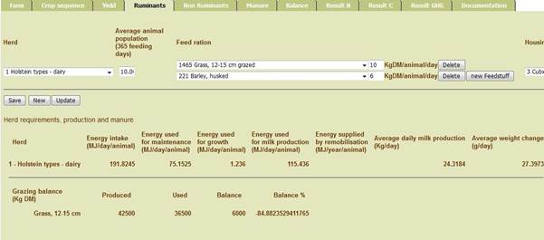
Fig 14 Defining the number and feed ration of ruminants

This tab also allows the type of animal housing used (if relevant) and the type of manure storage (Fig 15). If the livestock are not housed at any point in the year, choose “None”.

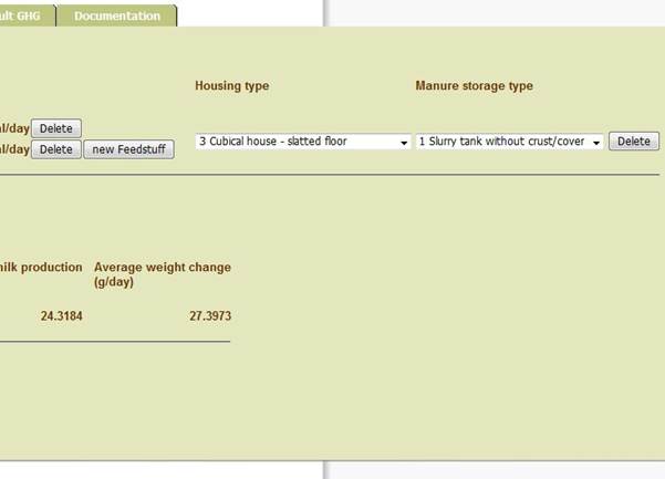
Fig 15 Defining the livestock housing and manure storage

Since the type of livestock housing determines the type of manure produced, the choice of manure storage varies depending on the type of housing chosen. If you change the type of housing, you need to allow time for the choice of manure storage type to be updated.

Table 6 Data inputs for each cattle type

User input	Description
Cattle type	Relevant type of cattle e.g. Holstein, mature weight 500kg
Number of cattle	Average number of cattle present
Livestock housing	Livestock housing type e.g. freely ventilated, fully slatted floor
Manure storage	Type of manure storage e.g. slurry tank (uncovered), slurry tank (covered)
Production	For dairy animals; milk production (kg yr^-1), for beef animals; average daily growth rate (g day^-1).
Type of feed item n	Type of feed item (e.g. high quality silage)
Amount of feed item n in the feed consumed	Amount of feed item consumed (kg DM animal^-1 day^-1)

The information allows the model to calculate the total energy consumption of each type of ruminant and how this energy is partitioned between maintenance, growth and/or milk production. Whenever the user clicks on the Update button, the modelled calculates the current energy intake and partitioning, enabling the user to adjust the ration to achieve the desired level of milk production and liveweight gain. Note however, it is the user’s responsibility to ensure that the feed ration can be consumed by the ruminants i.e. that the digestibility of the ration is sufficiently high.

The information input allows the model to calculate the DM, C and N consumed by each category of ruminant and the partitioning of that C and N between production (milk and growth) and excreta. The excreta C and N is further partitioned between the C and N deposited on fields during grazing and the C and N deposited in animal housing. The proportion of the C and N excreted partitioned to the fields is equated to the proportion of the total DM intake that is obtained by grazing.

4.6.1 Grazed feed items

Particular care needs to be taken over inputting grazed feed items, since the consumption and production must balance. Clicking the Save button prompts the model to calculate the production of grazed feed items (from the data entered on the Cropping sequence and Yield tabs) and the consumption of these feed items by the livestock. The results are displayed at the bottom of the tab in terms of the production and consumption of each grazed feed item, the absolute balance (production – consumption) and the relative balance ((production – consumption)/production). The user must ensure that the production and consumption of each grazed feed item equal one another, within a margin of error. The margin of error allowed is normally set at 2% or (for very low production systems) 50 kg DM.

4.7 Non-ruminant tab (currently only pigs) Not currently functioning

The Non-ruminant tab allows the user to input the number of sows, a number of piglets weaned per sow, the weight of the piglets at weaning, the annual energy requirement and the feed ration (type and amount of energy supplied).. For piglet and finisher production, the production is expressed in number of animals produced per year, rather than the annual average population. To calculate the number of animals produced per year from a measurement of the annual average population, it is necessary to divide the annual average population by the number of production cycles per year. For piglet and finisher production, the start and end weight, the energy required to produce a single animal and feed ration must be input. The user will be warned if the energy supplied in the feed ration is insufficient to meet the energy requirement input of the user. The user then has the opportunity to either change the production level or the feed ration. (In the longer term, we should allow the definition of a feed ration, as for cattle).

The type of animal housing used must be input for all pig types. For piglet and finisher production, a single animal housing type is assumed whereas for the sows, the housing types for pregnant and lactating sows are entered separately.

The information input, plus information on the N content of the elements included in the feed ration, allows the model to calculate the dry matter and N consumed by each category of pig and the partitioning of that N between growth, urine and faeces.

Table 7 Data inputs for each pig type

User input	Description
All pigs
Livestock housing	Livestock housing type or types e.g. ventilated, fully slatted floor
Manure storage	Type of manure storage e.g. slurry tank (uncovered), slurry tank (covered)
Sows
Number	Average number present
Number of piglets per sow	Number of live piglets per year
Weaning weight of piglets	Weaning weight in kg
Type of feed item n	Type of feed item (e.g. soya, barley)
Amount of feed item n in the feed consumed	Amount of feed item consumed (kg DM animal^-1 day^-1)
If the model is not coupled	Relevant housing types
Amount of feed item n offered	Amount of feed item supplied (kg DM animal^-1 day^-1)
Other types of pig
Number	Number produced per year
Start weight	Starting weight of this category (kg)
End weight	Finishing weight of this category (kg)

4.8 Manure tab

The manure tab lists each crop in each Cropping sequence. The user must input the amounts of manure or fertiliser applied to each crop and when the application is made. More than one type of manure or fertiliser can be applied to a given crop. For the manure, the application method must also be indicated. This will be via a drop-down box that will allow the user to indicate an application method appropriate for the manure type (e.g. broadcast application, slurry injection for liquid manure; surface application with no incorporation, surface application with incorporation within 6 hours for solid manure) (Fig 16 and Table 8).

Fig 16 The Manure tab

Table 8 Data inputs for manure and fertiliser applications

User input	Description
For each crop
Manure/fertilizer type n	Relevant manure/fertilizer types e.g. cattle FYM, ammonium nitrate, urea
Application technique/spreading method	e.g. slurry injection, broadcast spreading, rapid incorporation
Amount of manure/fertilizer n	For manure; m³ ha^-1, for fertilizer; kg ha^-1 N
Timing of application of manure/fertilizer type n	Month

A manure account is presented at the top of the Manure tab. This shows the amount of manure N that the model calculates (by clicking Update on the Ruminants or Non-ruminants tab) and the amount that has so far been allocated for field application. This information is useful if the export of manure from the farm is known, since it allows the field applications to be adjusted until this value is achieved. If inputting manure data for a farm for which empirical data are available, it is likely that these empirical data will have other units than kg N ha^-1. In this case, the N contained in one of these alternative units should be calculated by dividing the total manure N production shown on the Manure tab by the total amount of manure applied, expressed in the alternative units.

4.9 Nitrification inhibitor

Nitrification inhibitor is applied using the fertiliser application input on the Manure tab. A single nitrification inhibitor (called "Nitrification inhibitor") may be chosen from the list. The text box normally used to input the amount of fertiliser is borrowed here to enable the initial efficiency of suppression of nitrification to be indicated; instead of kg/ha, the reduction efficiency should be input as a proportion (i.e. should have a value between 1.0 and 0).

The efficiency of the nitrification inhibitor is assumed to decrease with time, due to degradation. The degradation rate is made a function of temperature (Fig 17).

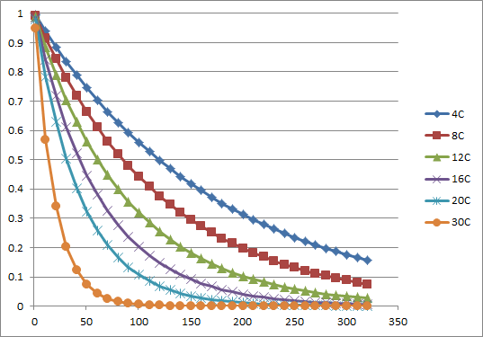
Fig 17 The reduction in the effectiveness of nitrification inhibitor with time

5 Running the model

Once the user has defined a baseline scenario, they should then return to the Farm tab and click on the Run model Adaptation button. The model will then be run in Adaptation mode. If the model generates an error, an error message will appear on the Farm tab (more information on the errors messages is available below), otherwise the user interface will switch to the Result N tab. The user should then return to the Farm tab and click on the Run model Projection button. Again, if the model generates an error, an error message will appear on the Farm tab, otherwise the user interface will switch to the Result N tab. The Result N, Result C and Result GHG tabs show the farm balances for N, C and greenhouse gases respectively. The Balance tab shows an overview of the manure and crop production and its fate. It is the responsibility of the user to ensure that the model has been configured correctly. In particular, this means that on the Balance tab that the desired import and export of roughage feed or manure has been achieved.

One or more alternative (non-baseline) scenarios can there be defined and simulated. For these simulations, only the Run model Projection button should be used.

5.1 Balance tab

The purpose of the balance tab is to give the user an overview of the use of feed items, crop products and manure.

For the manure, the mass of N produced, bought/imported, sold/exported and used is shown.

Each crop product produced or used on the farm is listed in a single column (Fig 18). To the right of this are four columns showing for each of the crop products the kg DM produced or used:

· The amount produced.

· The amount bought/imported.

· The amount sold/exported.

· The amount consumed by livestock or used as bedding.

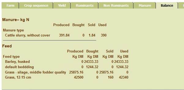
Fig 18 Example of the Balance tab

The user should use the Manure tab to ensure that the import, production, export and use of crop products and manure are consistent and coherent. This may require the user to adjust one or more of the following: the N applied to the crop (e.g. amount of N fertiliser, entered in the Manure tab), the production estimate or the type of crop product (entered in the Yield tab), or the livestock feed rations.

It is the responsibility of the user to ensure that the type of crop product produced is consistent with the cropping practice (climate, length of the growth period, mineral N supply etc). In particular, the user needs to be aware that the model has no automatic mechanism for changing the protein (N) concentration in crop products, in response to changing N supply. Note that changing the yield of crop that is grazed will also require a subsequent adjustment of the feed ration of the ruminants that are doing the grazing.

5.2 Result N and C tabs

The Results N and C tabs show the farm N and C balances calculated by the model (Fig 19). The difference between the N or C entering the farm and the N or C leaving the farm (farm N or C surplus) is partitioned between the loss pathways. Increases or decreases in the N and C stored in the soil are shown as positive or negative values respectively. The balances are displayed in two forms; farm totals (kg yr^-1) first and below them, per unit area (kg ha^-1 yr^-1).

Fig 19 Example of Results N tab

The Results N tab also contains links that allow the user to download a number of result files (Table 9). To download these files, point the computer mouse at the link, right click and select “Save link as….”.

Table 9 Detailed result files that are downloadable from the Results N tab

Link to file	Format	Content
Livestock file as xls	Excel	Details of the livestock DM, N and energy intake, production and excretion
Livestock file as xml	XML
Result as xml	XML	Detailed results at the farm scale plus key results for all farm components
Result as xls	Excel
Ctool as xls	Excel	Details of the C and N dynamics in the soil
Ctool as xml	XML	Details of the C and N dynamics in the soil
waterDebug	Excel	Details of the water budget

At the moment, we have no detailed description of these files.

In addition, the results of the simulations of the Crop sequences can be seen by clicking on ‘graphs’.

The ResultsC tab shows the equivalent results for C flows.

5.3 GHG tab

The Result GHG tab show the GHG emissions and a diverse range of production and environmental indicators. The greenhouse gas emissions, measured in CO₂ equivalents, are presented for each of the following (Fig 20):

Direct GHG:

· Enteric methane emissions

· Manure methane emissions

· Manure N₂O emissions

· Field N₂O emissions

· Change in C stored in soil

· Total direct GHG emissions

Indirect GHG:

· Housing NH₃ emissions

· Manure storage NH₃ emissions

· NH₃ emissions from field-applied manure

· NH₃ emissions from fertilisers

· N₂O emissions resulting from leaching of N

· Total indirect emissions

Fig 20 Example of Results GHG tab

6 Correcting errors

There are a number of types of error:

· Logic errors. These are errors in the logical description of the farm. For example, if you have indicated that a crop will be grown between April and August but also indicate that manure is applied to the crop in March. These errors will normally be trapped by the web interface or be explicitly named in the error message you will receive. The error can be corrected via the web interface.

· Technical errors. These occur when the model is unable to read input from one of the parameter files. An example would be if you have made a typographic error when editing a parameter file (e.g. input a value of 0.00.9 instead of 0.009). This error will normally result in an error message that is long and impossible for you to interpret. If you have previously run the model successfully, you need to look at the parameter files you have edited.

· Model errors. These occur because of an error in the model itself. We hope that we have now run sufficient scenarios that this is unlikely to occur. If it does then email us.

· Grazed yield error at the crop scale. This occurs when the crop submodel was not able to produce the grazed product yield that you indicated on the Yield tab. The crop sequence and crop name will be reported in the error message. The solution is to either reduce the amount of grass grazed or increase the production (see below).

· Grazed yield error at the farm scale. This occurs when the total farm-scale production of a grazed product differs too much from the total consumption of that product by the livestock. The solution is to either reduce the amount of grass grazed or increase the production (see below).

The commonest error is that the crop submodel was not able to produce the grazed yield of one or more grazed crop products. You now have three choices:

· Reduce the grazed yield of the relevant crop product (on the Yield tab) and reduce the consumption of that product (on the Ruminants tab).

· Choose an alternative crop product, one that has a lower concentration of protein (lower protein = higher dry matter yield per unit of N available from the soil).

· Choose to irrigate the crop. This is only relevant if you think that the crop production is limited by water availability (you can try using irrigation to see if this solves the problem). This option will not be available if you know that a crop is not irrigated.

· Increase the supply of N to the crop (on the Manure tab). This could mean reducing the application to one or more other crops or by applying fertiliser/imported manure.

When you have made changes, you should go to the Farm tab and click on the relevant Run model button again. You may have to repeat this cycle of run – error – correction – run.

7 Adaptation of soil model

The FarmAC soil model contains three C pools; Fresh organic matter (FOM), which is readily-degradable organic matter added to the soil in crop residues and manure, Humus organic matter (HUM), which is more stable organic matter and Resistant organic matter, which is almost completely unavailable to soil microorganisms. The FOM, HUM and ROM degrade rates that mean that the C in these pools has a half-life of about 6 months, 37 years and 1500 years respectively. The stable nature of the ROM means that it is only of importance when considering long-term land use change and is virtually irrelevant when considering relatively short-term changes in management. In the AnimalChange project, we are mainly concerned with changes in C sequestration over periods of 10 to 100 years, so we can afford to ignore the ROM pool.

The objective of the initialisation of the soil model is to bring the amount of C in the different pools to levels that reflect the previous land use and management history of the farm concerned.

There are two situations that we can recognise:

3. Farming systems where there has been no dramatic changes in land use in the past hundred years (e.g. from forest to agricultural land) and the cropping practice and management has been relatively stable over the recent past 50 years (e.g. has been grassland or arable during this period). Here we can assume that the soil C pools of interest are largely in equilibrium with the inputs of crop residues and animal manure.

4. Farming systems where there has either been a change in land use in the past hundred years (e.g. from forest to agricultural land) or a substantial change in the cropping practice and management over the past 1-50 years (e.g. from grassland to arable or the reverse). Here we must assume that the soil C pools of interest are not in equilibrium with the inputs of crop residues and animal manure.

7.1 Case 1 – soil in equilibrium with land use and management

For case 1, the situation shown in Fig 21 can be envisaged as an example. In the adaptation period, the aim is to enable the soil model to reach an equilibrium state in relation to the current (baseline) management. This can be achieved by simulating several hundred years with the baseline management. The period of adaptation is set by the adaptationTimePeriod parameter in the constants.xml file and has default value of 500 years.

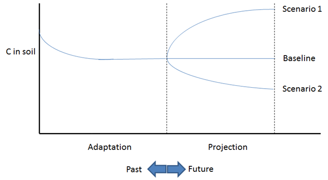
Figure 21 Changes in the C in the soil of a single crop sequence; soil is in equilibrium with management at the end of the adaptation period.

At the end of the adaptation period, the projection scenarios are imposed. The model is then run with the soil model for each crop sequence initialised to the average equilibrium condition for the soil on the farm. The farm-scale C and N flows and the production characteristics are averaged over the projection period. The projection period is set by the minimumTimePeriod parameter in the constants.xml and has a default value of 10 years.

Note that if there more than one crop sequence on the baseline farm share a soil type, the soil conditions used for initialising the soil model for the projection period will be the area-weighted average of all crop sequences. This is because the user may choose to change the area associated with the different This means that in the projection period, crop sequences in the baseline situation will usually experience changes in the amount of C stored (though the average change on the farm will be zero).

7.2 Case 2 – soil not in equilibrium with land use and management

For case 2, the situation in Fig 22 can be envisaged. In these cases, the values used to initialise the soil model in the baseline scenario must be those appropriate for the equilibrium situation for the historical land-use or management. The baseline land-use and management must be imposed. The baseline scenario must then be run for the adaptation period. The projection scenario is then run, initialising the soil model with the values obtained at the end of the adaptation period.

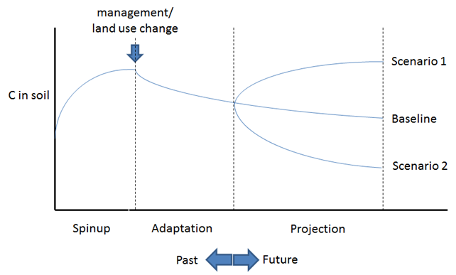
Fig 22 Schematic representation of the changes in soil C during spinup, adaptation and projection

7.2.1 Step-by-step instructions

1. Create a farm scenario that describes the land use/management in the past (prior to the change to the baseline management).

2. Press the ‘Adaptation’ button on the Farm tab and run the model.

3. Download the ‘Ctool result as xls’ file and use the final states of the FOM, HUM and ROM pools to initialise the C-Tool parameters for each soil type present, for the farm type to be used in the baseline scenario*.

4. Create a baseline scenario.

5. Modify the constants.xml file so that the spinupYears parameter equates to the adaptation period and the minimumTimePeriod equates to the projection period. Upload this to the server.

6. Press the ‘Adaptation’ button on the Farm tab and run the model (making corrections if necessary).

7. Press the ‘Projection’ button and allow the model to run again with the baseline scenario. Note the results (or download the results file(s)).

8. Create your projection scenarios. Do not include the text ‘baseline’ in the scenario name.

9. For each projection scenario, press the ‘Projection’ button and allow the model to run (or correct any errors and then run the model again). Note the results (or download the results file(s)).

* InitialC = FOM + HUM + ROM, pHUMupperLayer = pHUMlowerLayer = HUM/(HUM+ROM).

8 Crop residues

8.1 Arable crops

Arable crops can often either be harvested as whole crop or at maturity. Harvesting as whole crop means stems, leaves and grain are harvested and stored as one product e.g. as a high-quality roughage feed for cattle. Harvesting at maturity leads to the production of two crop products; grain and straw. The choice of which products should be produced from a given crop is made on the Crop sequence tab. The choice of crop products, like the choice of crops themselves, varies between different Agro ecological zones. For some crops, there is a choice of the quality of the product or products produced. It is the responsibility of the user to ensure that it is realistic to expect that the crop can produce these products under the climatic, soil and fertiliser conditions imposed. Note that it is also the responsibility of the user not to make impossible choices e.g. to select whole crop has Product 1 and then select Product 2 to be anything other than None.

The grain is always harvested whereas the choices for the fate of the straw varies between crops. For all crops, the straw can be harvested or incorporated into the soil. For some crops, there are additional options (Table 10).

Table 10 Fate of straw products

Straw use	Fate of straw product	Notes
Harvested	Straw is harvested and removed from field. Stubble is incorporated in the soil surface at harvesting time.	Available for all crops that produce straw
Incorporated	As for Harvesting (incorporation to depth not currently implemented)	Available for all crops that produce straw
Burnt	All straw is burnt; no stubble remains to be incorporated in soil
Burnt stubble	Straw is harvested and removed from field. Stubble is burnt.
Residue grazed, stubble burnt	Straw remains as a residue and is grazed during the subsequent crop. Any residue remaining ungrazed is burnt	Only available if the subsequent crop is bare soil
Residue grazed, stubble left	Straw remains as a residue and is grazed during the subsequent crop. Any residue remaining ungrazed is incorporated in the soil surface	Only available if the subsequent crop is bare soil
Residue grazed, stubble incorporated	As for Residue grazed, stubble left	Only available if the subsequent crop is bare soil

The choice of the fate of the straw product is made on the Yield tab. If the Straw use of a crop is set to produce residues, the user interface includes a drop-down product box for the following bare soil crop on the Cropping Sequence tab and a yield box for Product 2 for the following bare soil on the Yield tab.

8.2 Grassland and other grazable crops

Grassland and grazable crops are a special case. Firstly, these crops can usually be grazed, harvested or both. The model allows for a maximum of two crop products. For most crops of this type, either of these two products can be grazed or harvested. However, for some crops (e.g. some extensively grazed native vegetation), there may be crop products that are not eaten and these are treated as if they were straw products (see Table 1 above). For a crop product to be grazed, its name must include the keyword ‘grazed’ in its name. Since grassland and other grazable crops can be harvested at different stages of maturity and hence quality, there will often be a large choice of possible crop products. As for arable crops, it is the responsibility of the user to ensure that it is realistic to expect that the crop can produce these products under the climatic, soil and fertiliser conditions imposed.

The provision of two crop products enables a variety of situations to be simulated:

· One product is grazed, the other is harvested for hay or silage.

· One product is grazed whilst the other is not.

· Both products are grazed or harvested but have different qualities.

If a crop product is grazed, the yield of the crop product must be input on the Yield tab. Within a certain margin, this yield must be achieved or the model will report an error. In addition, the total yield of this product (which could be produced within a number of crop sequences) must match the total consumption of the product by the grazing animals. This restriction is necessary to ensure that the C and N flows within the farm are consistent. Note that for grazed crop products, if the modelled yield exceeds the value input on the Yield tab, the excess yield will be considered as crop residue by the model and returned to the soil.

9 Tips and tricks

9.1 Plotting the contents of result files

In the longer term, we hope to include plotting functions in the user interface. At present however, there is the option of using two macro-enabled Excel files developed during the AnimalChange project to plot some of the contents of the results files. These Excel files can be downloaded from the web interface.

9.1.1 Plotting soil C dynamics

1. From the Results N tab on the web user interface, download the CTool results file (right click on “Ctool result as xls” link, select “Save link as …” and save the file to your PC*).

2. Open the Excel spreadsheet called “Spin v3.xlsm”.

3. Go to the Control tab and enter the name of the directory where you saved the CTool results file.

4. Enter the name of the CTool file that you saved (us Ctrl-v if you saved the filename in the Clipboard)

5. Type Ctrl-r and the data will be copied into the spreadsheet and results plotted as graphs. The data from Crop sequence 1 will appear in worksheet Data 1 and the plots in Fig 1 etc.

* if when you save the file, you copy the filename into the Clipboard (Ctrl-c), you can paste the filename later.

Note: if you decide to save the plotted results in a new file, make sure that the name of the new file contains the text “spin” if you think you may wish to use the macro to replot the data at a later date.

9.1.2 Plotting crop dynamics

1. From the Results N tab on the web user interface, download the crop results file (right click on “Cropresult as xls” link, select “Save link as …” and save the file to your PC*).

2. Open the Excel spreadsheet called “CropPlots v2.xlsm”.

3. Go to the Control tab and enter the name of the directory where you saved the crop results file.

4. Enter the name of the crop results file that you saved (us Ctrl-v if you saved the filename in the Clipboard)

5. Type Ctrl-k and the data will be copied into the spreadsheet and results plotted as graphs. The data from Crop sequence 1 will appear in worksheet Data 1 and the plots in Fig 1 etc.

* if when you save the file, you copy the filename into the Clipboard (Ctrl-c), you can paste the filename later

9.2 Preventing the model averaging the soil conditions of a single soil type

When the baseline scenario is run in the Adaptation mode, a file is created that contains the final status of the soil model pools for each soil type. This means that if the same soil type appears in more than one crop sequence, the final status will be calculated as the area-weighted average. This is because the user may wish to alter the distribution of areas between crop sequences. This means that whilst the soil model is in equilibrium with the management at the farm scale, it may not be at the scale of the crop sequence. For example, if the farm had one soil type and in the baseline scenario, there are three crop sequences, the soil model in the scenarios would be initialized with the area-weighted average conditions at the end of the adaptation simulation. This is despite there probably being differences resulting from the different management applied to these crop sequences. This is necessary because the user may choose to adjust the relative areas of the different crop sequences and the model has no mechanism for identifying how this rearrangement occurs. If a user does not wish to adjust the areas of the crop sequences and a soil type is present in more than one crop sequence, it is possible to prevent the model from taking the area-weighted average. This can be done by selecting a different soil type for each crop sequence and then editing and uploading the parameter.xml file so that all these chosen soil types have the same characteristics. In essence, this deceives the model into treating the soils as different types, even though they have exactly the same characteristics.

9.3 Work-arounds for special situations

9.3.1 Feeding crop residues

At present, the user interface is unable to recognize crop residues when the user selects the cattle diet. As a temporary measure, the following substitutions can be made and will be converted in the code:

acidified milk = grazed residue millet hay (feedCode 310 to converted to feedCode 925)

whey = grazed residue groundnut hay (feedCode 312 converted to feedCode 926)

willow foliage = grazed dry fallow grass (feedCode 254 to converted to feedCode 934)

9.3.2 Corralling cattle

The model partitions the C and N excreted by animals between animal housing and one or more grazed fields in proportion to the dry matter intake of the feed items. In a situation where cattle are both housed and the grazed, any imported feed it is assumed to be fed in the animal housing. So in this case, if category L have a feed ration consisting of a single imported feed item and a single grazed feed item that is produced by two crops ( 1 and 2), the partitioning is as follows:

N deposited in housing = N excreted by L * imported feed item DM consumed by L/total DM intake by L

N deposited during grazing = N excreted by L - N deposited in housing

N input to crop 1 = N deposited by L during grazing * (DM production of grazed feed item by crop 1/total DM production of grazed feed item)

Likewise for crop 2.

If the livestock are not housed, the excreted N is distributed as follows:

N input to crop 1 = N excreted by L * (DM production of grazed feed item by crop 1/total DM production of grazed feed item)

Likewise for crop 2.

If the livestock are corralled overnight on a field, the assumption underlying the distribution of excreta will be incorrect. However, the model can be fooled into simulating the situation if the proportion of grazed DM production on the corralled field is made artificially higher than in the remaining fields. This can be achieved even if there is a significant intake of grazed forage or residues on other fields. This is achieved by considering most of the grazed DM production to be cut and fed to the livestock. Provided the parameterise determining processing and storage losses for the relevant products is set to 0, all the C and N in the products will be available for consumption and since there is no housing, all the associated excretion will be deposited in the field. A small amount of grazed product is then included in the diet and the production of this small amount of grazed product is distributed between the corralled crop and any other grazed crop in such a way that a disproportionately large amount occurs on the corralled crop.